

ABSTRACT
Tunnel boring is essential for many construction projects, yet it is challenging to accurately forecast productivity due to many influencing factors including ground conditions. Whilst ground survey data has improved over the years, significant gaps will always remain due to the inability to carry out boreholes for every metre of the tunnel. Accurate forecasts are essential for project management and can help to identify potential excavation challenges, manage stakeholders, and ensuring a confident forecast.
Murphy Group engaged me to develop and apply artificial intelligence to tunnel boring, specifically to forecast tunnelling progress. The algorithm selected for this study was a neural network, which is an algorithm that can learn patterns from real-world data that are non-linear, complex, and incomplete. Such data are characteristic and prevalent within soil-tool interactions, making neural networks a case study worth investigating.
The work in this paper shows two case studies.
The first was on a prior project – Southwark Tunnel, in London – which provided an array of machine sensor data. The project data would help in this first case study by enabling understanding of how well neural networks can capture tunnelling performance and machine behaviour, based on the performance data from the tunnel boring machine (TBM) on that project.
The second case study would take forward development of the neural networks by further applying the system to a live tunnel project, the North Bristol Relief Sewer (NBRS), and this time by only using geological data. This approach was designed to mimic the situation of data availability at the pre-tender stage of a project, where having such a system to support making a reliable forecast on tunnelling progress would have been valuable to a business looking to bid on such a contract.
The results of the studies showed neural networks to be successful at forecasting tunnel boring completion and the system was also able to capture spikes in excavation performance. This was particularly impressive as the spikes captured were from geological data points not been previously collected: gypsum and sandstone.
Additionally, neural networks demonstrated excellent generalisation when applied to Southwark Tunnel and were again able to accurately forecast the behaviour of the TBM. This project demonstrated the feasibility of artificial intelligence and highlighted promising applications in tunnel boring to address productivity and improve efficiency, which are both being taken forward by Murphy into further work.
INTRODUCTION
Project Background
I studied an MEng in Product Design Engineering at Loughborough University, with a placement year at JCB Excavators as an engineer. I later pursued a PhD in Artificial Intelligence for Robotic Excavation, and it was at this time that I gained interest in tunnelling. Despite having no tunnelling experience at the time, I was driven to apply my newfound skillset in artificial intelligence to tunnelling.
Murphy Group engaged with me to undertake a study to investigate the feasibility of machine learning for forecasting tunnelling. This is a new area for Murphy Group, as well as the tunnelling industry, but the potential benefits are numerous, with more accurate, data-driven forecasting the main benefit.
The TBM used in this exercise – for both projects discussed – was an earth pressure balance (EPB) Lovat RMP131SE machine, capable of building a 2.85m i.d. lining. The EPB machine is shown in Figure 1.
Murphy Group were engaged on the NBRS project for Wessex Water during the period of this work. The project had been awarded in early 2018 and involved construction of a 5.5km-long, 2.85m i.d. tunnel, requiring excavation of two 30m-deep 6m-i.d. shafts, 14 manholes, 1km of pipe jacking and auger boring drives, and 1km of open cut digging for pipework.
The ground was predominantly mudstone, siltstone, and conglomerate.
Murphy Group also had the tunnelling data for Southwark Tunnel, a previous tunnelling project undertaken that involved construction of a 9.0m diameter shaft along with the 3.0km-long 2.85m i.d. tunnel.
I decided to use the Southwark Tunnel project as a proof-of-concept study prior to its further development on the NBRS. The Southwark Tunnel data included TBM data, which can be used to explore additional data science applications. The project involved excavation below the River Thames at depths of circa 30m, and the tunnel featured a minimum curve radius of 150m. The primary ground conditions were London Clay, Chalk, and the Lambeth Group.
What is Machine Learning?
A technology that can improve civil engineering’s efficiency is machine learning.1 This is a field of artificial intelligence that fits data onto a model to understand its underlying patterns, effectively learning from data over time.
By using such data-driven approaches, complex behaviours can be captured, even predicted.
The arrival of vast amounts of data, powerful computers, and a resurgence in artificial intelligence research has led to machine learning becoming a powerful tool in multiple industries.
Whilst sectors like automotive2, healthcare3, and finance4 are active in machine learning, construction has only recently begun to adopt artificial intelligence in select applications5. One of the primary applications is machine vision, which is predominantly used for safety 6, however research in construction output is lacking and there is ample opportunity to leverage the new technology.
Studies have been conducted that use machine learning to predict certain aspects of tunnelling performance.7,8 However, a key limitation of these is that they are inputted with the machine parameters, which are data that can only be used once a project has commenced.
Another limitation is that these methods rarely forecast sufficiently far ahead on a project, such as to the end of tunnel excavation. Instead, they are focussed on predicting the duration of the current ring being erected. This presents an opportunity to apply machine learning to tunnelling by focusing on the geological aspect and, further, to then apply it to tendering, improving the understanding of a project’s potential productivity and challenges.
Geology is difficult to predict, as only a snapshot is available at the tender stage of a project, but new modelling techniques like neural networks could be used to build an understanding of the ground conditions.9
Neural Network Theory
Neural networks are one of the most popular machine learning algorithms as they can handle multiple types of problem (such as regression and classification), yield high accuracy, and can be updated as new data are discovered.
One of the most popular applications for neural networks is object detection, with facial recognition on a phone being a prime example.
Neural networks are inspired by the brain, which itself is made up of neurons – signal transmission pathways. Here, for modelling analysis, ‘neurons’ are mathematical functions – algorithms – that accept weighted inputs, sum them, pass them through an activation function, and output a result. The networks are made from several such ‘neurons’ connected together.
Figure 2 shows a typical neural network structure.
To learn, a neural network adjusts the weights of each neuron input. This is performed during training, using a process called backpropagation:
- A data point is passed forward through the neural network to generate a prediction at the output.
- This prediction is compared to the actual value of the data at that point to generate an error.
- The error is moved backward through the neural network, slightly adjusting the weights of each neuron input. The size of this adjustment is known as the learning rate.
- The same data point is passed forward again, generating a slightly closer prediction.
- This process is repeated until the weights yield predictions that are close to the actual values.
It is important to not use all the available data for training the neural network as neural network performance needs to be validated by testing it on data it has never seen before, to ensure that it has captured the underlying patterns of the data. This train-test split is usually 70:30, as this provides the neural network with enough information to generalise across new datasets without relying on memorising the data, which is called ‘overfitting’. The impact of training is shown in Figure 3.
Scope of the study
Having established its potential benefits, regarding understanding productivity, Murphy Group was interested in applying machine learning for tunnel boring yet wanted to understand its capabilities and possible applications. The research question it wanted addressed was: What is the feasibility of machine learning to forecast tunnelling performance?
This question was addressed by the first case study, on the data from Southwark Tunnel. The study had the aim to: investigate the feasibility of neural networks for predicting multiple types of output, using both machine and geological data.
Next, there is a gap in the literature that needed to be addressed – projecting tunnelling performance without TBM performance data.
Current literature relies on TBM performance data that have been generated already in specific ground conditions. When the ground conditions are new, there are not much data. How the machine behaves in these conditions is unknown, requiring additional prediction and potentially lower predictive accuracy. Instead, the data available are the ground conditions and the tunnel plan. This led to my second case study, at NBRS, with the aim to: use a geology-based approach for forecasting the tunnelling productivity.
These aims were chosen to utilise new technology in a novel application that would help improve the efficiency of a tunnelling project by providing datadriven solutions to understand productivity. This project adds value by addressing a gap in the literature, building on existing research.
METHODOLOGY
Datasets
Datasets from two studies were used to train the neural networks.
The first study is Southwark Tunnel and the input data is summarised in Table 1 which contains TBM performance parameters, as used in previous literature.
A use-case for the Southwark Tunnel data is to look at on-going excavation works and machine behaviour analysis. A model built on TBM performance data can help improve the operating parameters of a machine in real-time, and future work could utilise this knowledge for machine automation. The flexibility of neural networks is demonstrated by predicting three different tunnelling metrics. There are also limited ground condition variables, meaning the model will have to accurately understand the machine.
The second study is from NBRS, with the data used summarised in Table 2. This was supported by Maxwell Geosystems ground survey data, which provided rich detail of the ground being excavated.
Maxwell was commissioned by Murphy Group to provide a 3D model that assigned a probability of each geology being encountered in 20m lengths along the tunnel. This resulted in the production of models that contained sections of the expected tunnel face with a confidence level of each geology to be encountered. No TBM performance data were used, making the primary use-case a forecasting project, and only ring cycle duration needed as a prediction.
Data preparation was required before the neural networks can be run. First, any missing datapoints had to be dropped as missing values can cause problems. It is better to drop data rather than to populate gaps as it is less likely to impact the training. Next, the data were scaled between -1 and 1, which allows different magnitudes of data inputs to be comparable on the same scale without losing the impacts of any changes. After an output is generated, it is rescaled to reflect its real-world value.
Training and Deployment
Both case studies have unique methodologies, due to their data train-test split requirements.
For the first case study, the model was trained on 1500 datapoints. One datapoint represents a 1m length of tunnel and 500 such datapoints were used to test the performance of the learning algorithm, where the model can make amendments to its parameters. Then, performance was finally determined on the remaining 950 datapoints, to ensure that the model had received sufficient data to capture the underlying patterns of the data.
Overtraining on the same data causes models only to memorise all the data hinders predictive performance. The training needs to be sufficient to ensure that the model can be generalised for application on new datasets, which a crucial aspect for real-world deployment.
For the second case study, the model was trained on 1000 datapoints, tested on 700 datapoints, and validated on 500 datapoints. These started from Ch.1021on NBRS project, which is at the start of the tunnel.
The dataset was used to train several variations of neural networks (‘machine learners’), across different parameters, until an accuracy of >85% was achieved and that best performing network was selected for deployment. If a future project is at the tender stage, a prediction can be made with the trained model. Additional training on new data will increase the accuracy, but the model at this stage will still be able to perform accurately, even when applied to new scenarios.
Three error metrics were used to assess performance of the neural network in both studies: Mean Squared Error (MSE); Mean Absolute Error (MAE); and, R2 correlation. These are all common for neural networks predicting numerical values and having three metrics ensures more robust decision-making. A value greater than 0.7 for these values is good.
MSE penalises high errors, making it useful for understanding how correct an answer is, and how common large errors are.
MAE, contrary to MSE, does not penalise high errors and is useful for understanding the actual spread of error of a prediction.
R2 is used to explain how well the inputs of a model can explain an output, like how correlation is used to explain relationships but in this case for a model. If R2 is >0.9, it means the inputs are likely too correlated to the output, meaning inputs are driving the output.
RESULTS
Case Study 1 – UKPN Southwark Tunnel
For the UKPN Southwark Tunnel dataset, the neural network that was used is detailed in Table 3. The neural network structure was selected based on initial experiments. The learning rate, batch size, and optimisation algorithm are all standard for this field. Training of the neural network started from Rings 1–2000, with predictions and further refinements then performed over Rings 2001–2950.
The neural networks were trained to output three parameters – Excavation Time, Excavation Rate, and Earth Pressure Balance – using a dataset with 11 inputs and 2950 data points. The dataset was predominantly of TBM performance data, which is useful for any running projects but should not be solely relied upon for a forecasting project, as the machine parameters will also need to be predicted. Table 4 has error results.
Excavation time for each ring was pleasingly accurate, even with uncertainty from other external factors such as breakdowns, with the machine learners able to capture the overall behaviour of the machine. Figure 4 shows a sample of the excavation time predictions, with previous actual data included to show how well the model continues a previous trend.
Here, a clear trend has been successfully captured by the algorithm. Even though there are significant deviations, as around Ring 2600, the overall MSE error metric is low (0.005). This means that, generally, the size of the error is low, as high deviations in prediction would be penalised.
The low error is again reflected by the MAE (0.06). As seen around Ring 2450, nuances of tunnelling performance are captured as shown by the dip in performance.
The error metric R2 (0.7) is lower than for the other two outputs, as there are fewer data sources that can help explain the behaviour of the algorithm. If the R2 value was >0.9, then the parameters of the TBM inputted are driving the outputs too high. This was not the case, as the R2 value was less than 0.9.
In future, additional data sources could be included to understand why there are deviations between the prediction and result. The prediction is also close to previous data points, as seen at the intersection, showing how it can accurately continue a previous trend.
Figure 5 shows the average excavation rate of the machine.
The average excavation rate results were even more accurate than the excavation time, with the behaviour accurately captured, especially after Ring 2600. This resulted in a low MSE (0.01), which was surprising considering the large deviation at Ring 2620 and after Ring 2550. The low error is best viewed after Ring 2700 and after Ring 2500, where the predictions are almost identical to the actual result. This low error is reflected by the low MAE (0.07).
Figure 6 shows the EPB predictions.
EPB was accurately captured, with only some deviation just before Ring 2600 and after 2400. This deviation was only slight, resulting in the lowest MSE of the three predictions (0.0009), and the error was not as common, resulting in the lowest MAE (0.02). EPB was able to be explained best by the sensor array used, as shown by its high R2 score (0.9). These predictions could be useful for predicting machine parameters needed, helping the operator to make more efficient decisions.
The results of the neural network were accurate and were able to capture the underlying behaviours of the machine. This was more impressive, as the neural network was simultaneously predicting three outputs (Excavation Time, Excavation Rate, EPB) which can impact the accuracy of the model.
Case Study 2 – NBRS Forecast
From training, the parameters of neural network used on the NBRS study are shown in Table 5. These were selected, based on trial-test methods and existing benchmarks, as seen in Case Study 1. The training data were from Rings 1000–2750, with Rings 2751– 3500 used for predictive testing. After training and testing, the model forecasted the remaining 2000 Rings of tunnel excavation.
One of the challenges was the prediction of Ring Cycle Duration. This was difficult to predict because of the variety within the data, as shown in Figure 7. Although the algorithm was able to anticipate spikes, there was a slight delay to the predictions and exact values were difficult to capture.
Here, there are frequent, irregular spikes within the data. Unfortunately, there may be several reasons as to why these outliers occurred.
For example, there could be breakdowns, the ground could genuinely be more challenging, production was stopped for grouting, or there was a new driver. Even so, the neural network showed promising performance in being able to at least anticipate harder conditions. This was especially clear around Rings 2871–2927, where a selection of difficult conditions was anticipated.
Although the predictions are slightly delayed by <5 rings, the behaviour could still be captured, which was useful for the team. More data would help to refine this further, especially to provide context to the data spikes. The model was trained on three months of data and forecasted five months work in total.
Additional challenges with the dataset were variables that the model had not been exposed to in training. This includes large amounts of gypsum and sandstone, which were mostly absent in prior training data. This means the impact from larger concentrations was unknown. Figure 8 shows the training data, and where it ultimately finished. After training, the model was compared to a benchmark provided by Murphy Group that was based on averages determined from previous excavations. This was approximately 60 rings per week.
To address this, bespoke algorithms for one output (as opposed to including EPB) were developed. More examples of outlier data were presented during the training phase to ensure the algorithms had more exposure on variable data. The output of the neural network is shown in Figure 9.
The model predicted high spikes, due to its anticipation of harder excavation from the sandstone and gypsum. This helped Murphy Group to prepare for these uncertainties. Interestingly, it was also predicting lower ring cycle durations than the proposed average. The model also predicted that the sandstone would be difficult to adjust to, noticeable between Ring 5033 and 5190. The behaviour of the machine in sandstone was accurately anticipated as it was reported that the sandstone was significantly harder to excavate yet was predicted with little available data.
Figure 10 shows the predictions against the actual results.
Here, the weekly forecast from the neural network was able to anticipate a decrease in productivity as the project ended yet maintained a weekly average that was often higher than the benchmark weekly production rate from Murphy Group. Although more data would help to further improve the predictive ability of the neural network, the forecast was significantly more accurate than the given benchmark, received on the same date as the neural network on 13 September 2021.
Whilst the existing benchmark predicted a finish in May, the neural network predicted a finish on 14 February 2022, within 14 days after the actual tunnel completion.
CONCLUSION
Neural networks demonstrated that they were able to understand the complex nature of tunnelling, and were able to yield accurate predictions, even with limited data. This was shown on two tunnel boring projects, in different ground conditions and with different datasets, demonstrating how generalisable the solution is. This is promising, as patterns could be anticipated in new settings, helping to form a more accurate tender, or to understand productivity as the tunnel is being excavated. Having a more accurate tender helps with budgeting, whilst being able to anticipate risk helps a project manager prepare for a mitigation.
Now that the neural network model is built, it can be applied to future groundwork projects to forecast the TBM performance in new ground conditions.
Murphy Group were satisfied with the results presented from the neural networks studies and is among the first to use machine learning in a tunnelling environment, as well as groundworks in general. Significant innovations in the field of artificial intelligence were made, as the current models have never been used to forecast such an ambitious output. Previously, machine learning researchers would rely on TBM performance data to help with the predictions. The approach proposed showed an innovative method that only used data inputs available at pre-tender.
By utilising the latest research, a successful industrydriven study was delivered.
The Southwark Tunnel model was able to predict the EPB, ring cycle duration, and rings per shift from the same neural network. The algorithm was efficient, yet still accurate, and is valuable for higher-level deployment.
Predicting machine parameters, such as EPB, is useful for autonomous projects, or as a driver-assist to recommend to an operator what controls they can consider for adjustment. The algorithm could also extract an innate understanding of the data without being heavily influenced by the operational data, as shown by R2 values being lower than 0.9. TBM data quality is important, as performance depends on data quality.
The NBRS model was shown to successfully forecast ring cycle time, a key metric for anyone planning or delivering a tunnelling project. It was also able to predict spikes and deviations, despite having no prior knowledge of the ground conditions.
The conditions that it lacked at training were sandstone and gypsum, but the neural network was able to correctly anticipate their impact.
The approach that this neural network used was novel as it didn’t use TBM performance data as inputs, meaning it could be used at the tendering stage.
There is opportunity to further improve the model by including the tunnel geometry, which may influence the performance. This can also be analysed to look for relationships between the geometry of the tunnel, ground condition and the time it takes to construct one ring. Data of unique ground conditions can be introduced, such as shear, moisture, and particle size. This would help enable easier training of a model, as it can find a relationship between the time to excavate and the ground conditions, with respect to other ground conditions.
The neural network could also be adapted for realtime project updates. By taking in machine parameters in certain conditions, projections can be adjusted. Collecting more of this data would also be integral for any future work that considers using data-driven technology to improve performance. By formulating a digital technology roadmap, with standardised, quality data at its core, multiple models for different tasks can be developed across the business, and the industry as a whole.
To conclude, this study demonstrated the successful application of artificial intelligence for tunnelling production forecasting. This was a novel use of a new technology that helped improve efficiency by understanding productivity by using a data-driven approach. Murphy is now taking further steps in this area to develop the work.